When developing software that makes use of a database, you may want to apply Agile principles to help tune your SQL queries. Simplicity, and being able to reduce the time scale of long running queries are the resulting benefits. In this article we discuss how to write more efficient code and reduce the overhead associated with long-running or inefficient queries.
When developing software that makes use of a database, you may want to apply Agile principles to help tune your SQL queries. Simplicity, and being able to reduce the time scale of long running queries are the resulting benefits. In this article we discuss how to write more efficient code and reduce the overhead associated with long-running or inefficient queries. The tool used is SQL Optimizer in Toad for Oracle XPert, but another tool may be used following a similar approach.
When developing SQL code for Oracle Database, or any other database, I often have some nagging issues surrounding the efficiency of the SQL. Is the SQL code the most efficient it can be? The objective is to run a SQL statement in the shortest possible time, avoiding excessive usage of resources (memory, disk, CPU, network). Specifically, the following parameters are optimized:
1. SQL Query Runtime – The time taken by a SQL statement to run.
2. Execution Plan - The sequence of operations performed to run a SQL statement.
3. CPU Usage – CPU used by a session. The less the CPU is used the more efficient the SQL query.
4. Session Logical Reads – Read requests for data blocks from the SGA.
5. Physical Reads – Actual reads to disk. A logical read results in a physical read if data is not available in the buffer cache. A physical read incurs a disk I/O overhead.
6. Sorts (Rows) – The total number of rows sorted.
7. Sorts (Memory) – The number of sorts made in memory. Memory-based sorts are more efficient than disk-based sorts.
8. Sorts (Disk) – The number of sorts made on disk.
9. Table Scan Rows Gotten – The cumulative number of rows read for full table scans.
10. Table Fetch by Rowid – The cumulative number of rows fetched from tables using a TABLE ACCESS BY ROWID operation.
11. First Row Time – Response time to fetch the first row, or the first n rows.
12. Parse Time – The CPU time taken for parsing
13. Table Scans – The Number of table scans. A table scan is the reading of every row of a table. Table scans are time consuming and can be avoided by using indexes.
14. Consistent Gets – A consistent get is a technique used to get data with which the data block is gotten from the buffer cache ensuring that the data block is gotten in a read consistent mode, i.e. the data block is current at the time when the query started.
15. Trace Statistics – Statistics on traced SQL statements
In this article we shall discuss how the SQL Optimizer in Toad for Oracle XPert edition could be used to optimize SQL statements.
Setting the Environment
The following are the prerequisites when using Toad for Oracle:
1. Download and install Toad for Oracle Xpert Edition, which includes the SQL Optimizer.
2. Create an instance of Oracle Database on either of the platforms: local machine, cloud platform. Oracle Database 19c is used in the article.
3. Create a connection to the Oracle Database in Toad for Oracle.
4. Select one of the default databases and a table within the selected database to use to run SQL statements. The SH.CUSTOMERS sample database is used in this article, as shown in Figure 1.
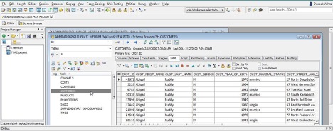
Figure 1. Selecting default schema and table as SH.CUSTOMERS
Launching the SQL Optimizer
To launch the SQL Optimizer, open an Editor window, and select Advanced SQL Optimizations (Figure 2) from the toolbar.
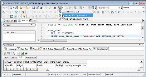
Figure 2. Selecting Advanced SQL Optimizations
In the Refactor SQL Before Optimizing dialog select the refactor options such as Correct WHERE clause indentation level and click on OK. In the Optimization Module Selector (Figure 3) select the module for optimizing SQL. If not sure about whether the SQL statement is well written, choose the Optimize SQL by SQL Rewrite module, which also provides index suggestions. To choose the best execution plan select the Optimize SQL by Plan Control module. And, if running batch SQL select the Batch Optimize SQL module.
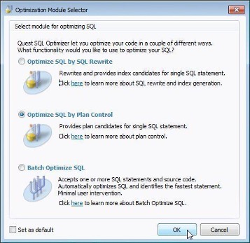
Figure 3. Select the Optimization Module
The SQL Optimizer gets launched (Figure 4).
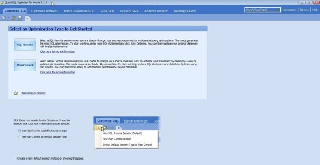
Figure 4. SQL Optimizer
Optimizing SQL
To optimize SQL, select the Optimize SQL tab (Figure 5), and select the Oracle database connection to use. Copy and paste the SQL statement to optimize in the Original SQL window:
SELECT /*+ ALL_ROWS */ cust_id, cust_first_name, cust_last_name, cust_email
FROM SH.CUSTOMERS
WHERE cust_first_name = 'Abigail' AND COUNTRY_ID=52770;
Click on the Auto Optimize using Plan Control link (Figure 3), which optimizes using the best execution plan.
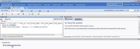
Figure 5. Optimize SQL
In the Test Run Settings dialog, select from the options listed to provide information about the SQL, such as Where the SQL is used, How the SQL is used, The execution frequency for this SQL, and Symptoms, and click on Start Test Run. The test run determines an execution plan for the SQL statement, which is displayed in the Execution Plan tab. Plan 1 is shown along with the Original SQL in Figure 6.
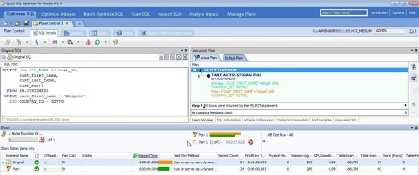
Figure 6. Execution plan along with Original SQL
To compare the Original SQL with the Execution Plan click on the Compare sub-tab (Figure 7).
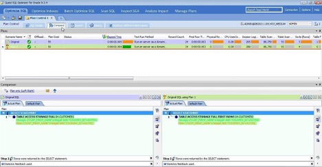
Figure 7. Compare the Original SQL with the Execution Plan
While getting details from the statistics displayed and making deductions may both be done by an expert DBA, I find it best to refer to the Optimize SQL Resolution Report (Figure 8), which is displayed with the Report sub-tab. As the Resolution Summary indicates in the first chart, The best SQL for Elapsed Time is Plan 1.
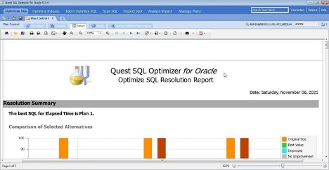
Figure 8. Optimize SQL Resolution Report
The Elapsed Time (Figure 9) is shown to have been reduced to 80% of the original SQL. The best execution plan is influenced by several factors and could be different for the same SQL code for different data volumes, bind variable settings (types and values), and initialization parameters and optimizer hints. Each time any of these is changed it is best to re-optimize the SQL code.
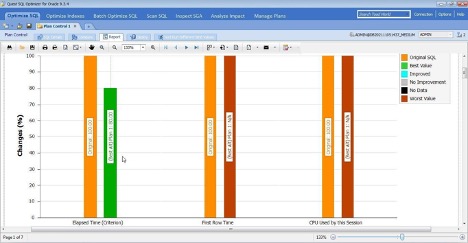
Figure 9. Elapsed time reduced to 80% of original SQL
I find that the bar charts make it easy to analyze the performance of SQL and choose the best alternative. While Elapsed Time Saved is 20%, no difference is noted for First Row Time, or CPU Used (Figure 10).
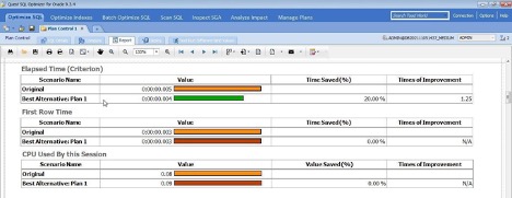
Figure 10. Bar charts
The Session Logical Reads, and the Physical Reads are compared in Figure 11.
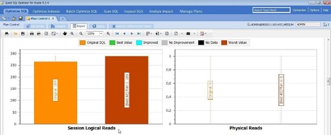
Figure 11.Session Logical Reads & Physical Reads
The Sorts (Rows) & Table Scan Rows Gotten are compared in Figure 12.
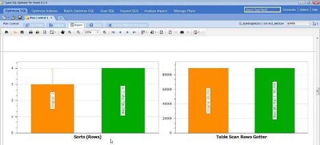
Figure 12. Sorts (Rows) & Table Scan Rows Gotten
Table Fetch by Rowid & First Row Time are compared in Figure 13.
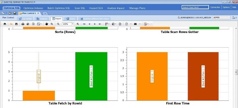
Figure 13. Table Fetch by Rowid & First Row Time
To test run different bind values select the Test Run Different Bind Values sub-tab.
Batch Optimizing SQL
If you have a batch of SQL statements to optimize, select the Batch Optimize SQL tab (Figure 14), and click on Add Code to Optimize.
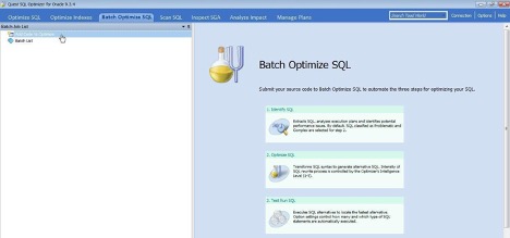
Figure 14. Batch Optimize SQL
Select a database connection in the Connection Manager. In the Add Batch Optimize SQL Jobs dialog, copy and paste the batch SQL to optimize in the SQL Text window (Figure 15). Select the Scan using Schema as SH. Similarly select the Execute using Schema as SH, and click on Next.
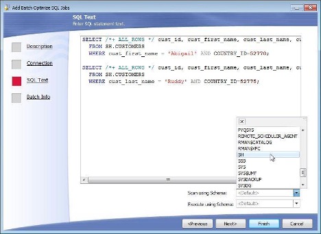
Figure 15. Add Batch Optimize SQL Jobs
Supply the Batch Info such as Batch Name, and click on Finish. The Cost and Elapsed Time Comparison chart (Figure 16) shows that this time no reduction in runtime, or elapsed time, is made between the original SQL and the fast alternative. To create a report, select Batch Job Report from the toolbar.

Figure 16. Batch Optimize SQL result
Scanning SQL
While we copied and pasted SQL, it is best to scan a more unwieldy SQL script using the Scan SQL tab (Figure 17). Click on Add Scan SQL jobs to add scan SQL jobs.
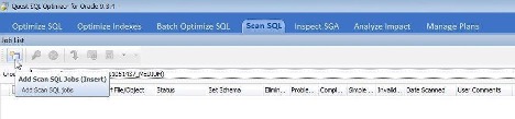
Figure 17. Scan SQL
First, select the Database Objects (Figure 18). Click on Next.
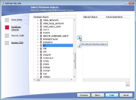
Figure 18. Select Database Objects
Next, select the source code to scan (Figure 19). For Source code type, select Text/Binary files. Oracle SQL *Plus scripts may also be scanned, or uploaded. In Add by file click on the + icon to select one or more text/binary files. Alternatively, to scan a directory click on the + icon in Add by directory. Click on Next to optionally inspect SGA, and click on Finish.
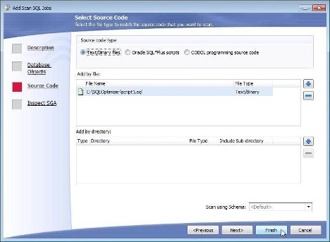
Figure 19. Selecting Source Code script/s to scan
The SQL code gets scanned, and an Execution Plan for the SQL gets displayed, but that is not all. To analyze the impact of changing SQL parameters on the scanned SQL, click on Send to Analyze Impact (Figure 20). Analyzing impact is discussed in the next section.
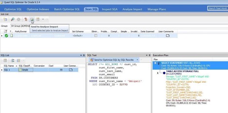
Figure 20. Send to Analyze Impact
To create a report of the scanned SQL, click on Scanned Job Report (Figure 21).
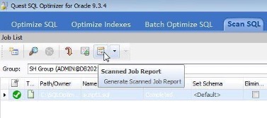
Figure 21. Scanned Job Report
Analyzing Impact
If you are given to tinkering with SQL parameters and optimizer hints to find how it affects performance, it is best to use the Analyze Impact feature. After selecting an SQL script to optimize, select the Analyze Impact tab (Figure 22), and click on the link in the Click here to modify parameter values.
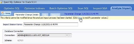
Figure 22. Analyze Impact
As an example, set the optimizer_features_enable hint, which enables a set of optimizer features based on the Oracle Database Release number provided as the value for the hint, in the Compare with value column to 18.1.0 as shown in Figure 23. The Compare from column displays the current value for the hint as 19.1.0.
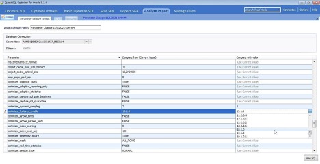
Figure 23. Setting value for optimizer_features_enable hint to compare
The impact of changing values for multiple parameters, or optimizer hints, may be analyzed in a single run.After changing the Compare with value for a few other parameters, click on View SQL (Figure 24).
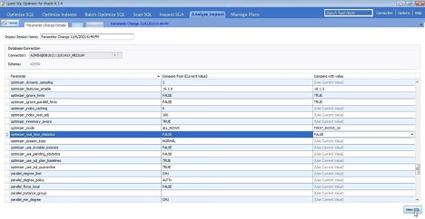
Figure 24. View SQL
The SQL Text on which the impact of making parameter changes is to be found, the SQL Summary, and the Parsed Execution Plan get displayed (Figure 25). Click on Finish to send SQL for impact analysis.
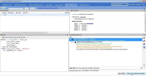
Figure 25. SQL to be optimized
An Analysis Impact Progress page (Figure 26) gets displayed. As the result indicates the “Impact Analysis completed with no impacted SQL found.”
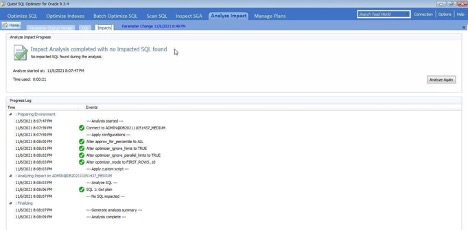
Figure 26. Analysis Impact Progress page

User Comments
Hi Thanks,
for sharing, it was informative.